Using GMYC for species delineation
About
This tutorial was written by François Michonneau with input from Matthieu Leray for the Marine Biodiversity Methods course taught at the Friday Harbor Laboratories, University of Washington.
This tutorial is released under a Creative Commons Attribution (CC-BY) license. It was originally published https://francoismichonneau.net/gmyc-tutorial, and can be cited using the DOI deposited at Zenodo:
Michonneau, F. 2016. Using GMYC for species delination. Zenodo. https://doi.org/10.5281/zenodo.838260
Background
To demonstrate how to use GMYC, we will use sequences from a sea cucumber species complex, Holothuria impatiens. These sequences are a simplified dataset from a real study that investigated this species complex to uncover that under the name Holothuria impatiens there were at least 13 species. For the sake of simplicity and efficiency, we will cut some corners, especially with the way we build the tree on which we will run GMYC but this example will demonstrate how to use GMYC and will easily be adaptable to other datasets.
GMYC (which stands for Generalized Mixed Yule Coalescent) is a very popular method that can be used to delineate species using sequence data. It uses an ultrametric tree and attempts to detect the transition in the tree where the branching pattern switches from being attributed to speciation (one lineage per species) to when it can be attributed to the intra-species coalescent process (multiple lineages per species). Therefore, for this method to work, the tree provided needs to be (1) fully resolved (without any mutlifurcations); (2) ultrametric (all the tips have the same age).
One way to obtain such a tree is to use the software BEAST. This popular and robust software for phylogenetic inference generates ultrametric trees. BEAST provides a very comprehensive framework for phylogenetic inference, but we will use only a few set of options for our purposes. BEAST uses a Bayesian framework for estimating the tree, and therefore returns trees sampled from the posterior distribution of the possible trees. We will need to summarize these trees to obtain a credible tree, that in turn we will use in GMYC.
Because BEAST uses a Bayesian framework, we will need to provide priors to be able to infer the topology and the branch lengths of the tree. Priors are an important component of Bayesian inference. They allow you to express your prior knowledge of the process you are attempting to model, reducing the number of options to explore, in turn maximizing your chance of getting the correct answer. However, deciding good priors in the case of a species delineation study is challenging because we need to model both processes that happen at the species level (speciation) and processes that happen at the population level (coalescent processes). Therefore, the correct choice for the priors is not always obvious. Methods are being developed to assess which priors are best suited for your data, but they are still very computationally intensive and a little impractical to use. In this tutorial, we will explore how the choice of the priors can affect the results of a GMYC analysis. We chose these examples to illustrate that you need to be mindful of the method you use to reconstruct the tree you will provide to GMYC.
There are other methods that can be used to obtain an ultrametric tree. They are typically done once the topology has been estimated by a phylogenetic method that represent the expected number of substitutions as their branch lengths (e.g., RAxML, MrBayes). However, they tend to not be as accurate as the joint estimation provided by BEAST.
In this tutorial, we will build 3 trees from the same DNA sequence alignment, by changing the priors we use with BEAST. In these 3 trees, the topologies will be very similar if not identical, however, the branch lengths will vary. We will vary two priors:
- the model used to express the expected branching pattern on the tree. We will
either use:
- a Yule model (also known as pure birth) in which all branching in the tree can be explained by a constant speciation rate.
- a Coalescent model with constant population size. This is typically the prior the most adapted to model the relationships among individuals from the same species.
- the rate of molecular evolution that we will model either as:
- a constant clock that assumes that mutations accumulates at a constant rate of evolution throughout the tree. This simplistic assumption works well when applied to related species, especially when a single marker is involved.
- a relaxed clock that assumes that rates of molecular evolution vary over the tree and are drawn from a statistical distribution. Here we will use a log-normal distribution (it is similar to a normal distribution but all values of the distribution are positive – we wouldn’t want to try to model negative rates of molecular evolution!). This is a good model to use if your tree includes many species, but you may need a lot of data to get accurate estimates of the parameters for this model.
We will thus build trees using:
- a Yule model and a constant clock that we will refer to as
yule - a Yule model and a relaxed clock that we will refer to as
relaxed_clock - a Coalescent model with constant population size and a constant clock
that we will refer to as
constant_coalescent.
Pre-requisites
Software
Please install the following software. They are all available for Windows, Mac, and Linux. However, some parts of this tutorial assume that you are using either Mac or Linux.
Files
- Aligned sequences:
impatiens.fasta
Estimation of the topology with BEAST
BEAST is a software package that comes with several tools. For this tutorial we will use:
- BEAUTI to prepare in the input file
- BEAST to run the analysis
- treeannotator to summarize the posterior distribution
Because we are going to test the effect of using different priors on the results of GMYC, we will generate 3 input files with BEAUTI.
Setting up the analysis with BEAUTI
The sequences provided here are already aligned, and are provided as a FASTA file. BEAST2 can directly import FASTA files.
Set up your analysis folder
Choose where you’ll store the results of your analysis on your hard drive. To keep things in order, we will create 3 sub-folders that will store each one of our analyses.
You should have the FASTA file at the root of this directory, and one folder for
each of the analysis we are going to carry based on the prior we will modify:
yule, constant_coalescent, and relaxed_clock.
Using a Yule prior
- Start BEAUTI
File>Import Alignment- Navigate to find the FASTA file for this exercise
- Go under the “Site Model” tab. We will use a HKY+Gamma model of molecular
evolution for this exercise. This is a simple molecular of evolution that
works well for this small dataset. On more complex datasets, you may want to
use a tool like
partitionfinder to identify
the most appropriate model of molecular evolution for your data. To do so:
- Change “Gamma Category Count” from 0 to 4. (Here we use 4 as it has been shown to be enough to capture most of the rate variation. On more complex datasets you can try to increase the number of categories to 6 or 10, see this paper for more information.)
- A “Shape” dialog box will appear, click on the “estimate” check box
- In the “Subst Model”, in the drop-down menu choose “HKY”
- Under the “Prior” tab, make sure the “Tree” parameter is set to “Yule model”
- Under the “MCMC” tab:
- change the “Chain Length” from 10 million to 5 million
- under “tracelog”, change the file name to
yule.log - under “treelog.t:impatiens”, change the file name to
yule_tree.trees.
- Save this file into your
yule/folder, and name ityule.xml
Using a Coalescent Constant Growth
To avoid mistakes and make sure our files only differ from each others by the prior chosen, we will copy the file we just created and modify the priors we want to adjust.
At the terminal, from the folder containing your FASTA files and the folder that will store the results of your analysis:
cp yule/yule.xml constant_coalescent/constant_coalescent.xml
cp yule/yule.xml relaxed_clock/relaxed_clock.xml
Now in BEAUTI:
File>Load, and choose theconstant_coalescent.xmlfile- Under the “Prior” tab, in the first drop-down menu, select “Coalescent Constant Population”
- Under the “MCMC” tab:
- under “tracelog”, change the file name to
constant_coalescent.log - under “treelog.t:impatiens” change the file name to
constant_coalescent.trees
- under “tracelog”, change the file name to
- Save the file (
File>Save) and Close.
Using a relaxed clock
In BEAUTI:
File>Load, and choose therelaxed_clock.xmlfile- Under the “Clock model” tab, in the drop-down menu, select “Relaxed Clock Log Normal”
- Under the “MCMC” tab:
- under “tracelog”, change the file name to
relaxed_clock.log - under “treelog.t:impatiens” change the file name to
relaxed_clock.trees
- under “tracelog”, change the file name to
- Save the file (
File>Save) and Close.
Double checking
At this stage your folder should look like this:
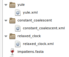
It is also a good idea to make sure that each one of your XML files are correct, so you may want to open them again in BEAUTI to check that all the parameters are accurate.
If you had trouble with making these files, you can download them below
Running the BEAST analysis
You can run this BEAST analysis on your computer. In this case, there are not too many sequences, and we don’t estimate too many parameters so it should take between 30 min and 1 hour to complete for each file. However, if you use a larger dataset, it may not be practical to run it on your own computer.
If your institution has a super-computer that you may use, it might be the solution that provides you with the most flexibility. Alternatively, there is a web portal that provides free access to a super-computer for phylogenetic analysis called CIPRES. CIPRES lets you run, free of charge, most popular phylogenetic software. There are limits on how long each analysis takes, but it should be enough for most analyses.
Where ever you end up running your analyses, it is always a good idea to check on your own computer that your input files are valid and that the run can start.
We will run BEAST from the command line as it provides more flexibility. At
the terminal, navigate to the yule/ folder and start your BEAST run:
cd yule
beast yule.xml
If everything goes well, after a few seconds, you should see something like this appearing on your screen:
===============================================================================
Start likelihood: -7518.152130664581
Writing file yule.log
Writing file yule.trees
         Sample      posterior ESS(posterior)     likelihood          prior
              0     -7518.1521              N     -7506.2589       -11.8932 --
           1000     -3469.6786         2.0        -3572.4855       102.8069 --
           2000     -2537.7958         3.0        -2666.2932       128.4974 --
           3000     -1958.7987         4.0        -2134.3332       175.5344 --
           4000     -1869.9440         4.5        -2046.0378       176.0937 --
This indicates that your analysis is running.
You will need to repeat this operation for the other 2 XML files
(constant_coalesent.xml, and relaxed_clock.xml).
To speed up the process so that you don’t have to wait for BEAST to complete, we are providing you with the output files for each of these analyses. Please make sure that you save these files in their appropriate folders:
- Yule: yule.log yule.trees
- Constant Coalescent: constant_coalescent.log constant_coalescent.trees
- Relaxed clock: relaxed_clock.log relaxed_clock.trees
Visualizing the posterior with Tracer
Explaining in detail how to analyze the output of a Bayesian inference is beyond the scope of this tutorial, but know that it is an important topic and that results should always be checked carefully before summarizing and analyzing them.
Start the Tracer program, and open one of your files (File > Import Trace
file). For instance for the yule.log, it should like:
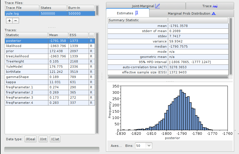
The exact numbers might differ for your analysis, as the results from a Bayesian inference are obtained through random sampling, and they may differ slightly between runs.
Tracer shows the mean values for the parameters used to infer the phylogeny. For the purpose of this tutorial we don’t need to get into the detail of what these numbers mean. However, an important source of information from this table are the values in the ESS (Estimated Sample Sizes) column. They indicate whether or not you can be confident that the values for the parameters are accurate. For an analysis that you aim at publishing, all the ESS values should be > 200. If they are not, it means that you should run your analysis longer (include more steps in your MCMC), or it might reflect an issue with your analysis such as over-parametrization.
Your turn:
Inspect the log files for your 3 runs.
Summarizing the posterior with treeannotator
Now that we confirmed that our analysis were adequate, we can summarize the
trees that have been samples from the posterior distribution into a single tree
that we can visualize. To do so, we will use the treeannotator program. We
will use the command line as it provides more flexibility. We need to run
treeannotator for each of the 3 analyses:
treeannotator -b 10 yule/yule.trees yule/yule_tree.nex
treeannotator -b 10 constant_coalescent/constant_coalescent.trees constant_coalescent_tree.nex
treeannotator -b 10 relaxed_clock/relaxed_clock.trees relaxed_clock/relaxed_clock_tree.nex
Each of these commands should take just a few seconds to complete and will produce a summary tree.
If you had trouble generating the trees with treeannotator, you can download the summarized trees below
- Yule: yule_tree.nex
- Constant Coalescent: constant_coalescent_tree.nex
- Relaxed Clock: relaxed_coalescent_tree.nex
Visualizing the trees with Figtree
We can now visualize the trees obtained for each of these priors. To do so, we will use Figtree.
Start Figtree, and open the files generated with treeannotator (with the
.nex extension): File > Open.
Your turn
Open the 3 tree files and compare them. How do they differ?
Estimation of the number of species included in the tree with GMYC
Now that we have our tree files, we can analyze them using GMYC.
Getting ready: installing the packages we’ll use
Before we can use GMYC, we need to install a few packages that will allow us to read the trees we generated in R, and do the actual GMYC analysis. Start R, and at the terminal type:
install.packages(c("ape", "paran", "rncl"))
install.packages("splits", repos = "http://R-Forge.R-project.org")
First let’s import in R the trees we generated with BEAST:
library(rncl)
yule_tr <- read_nexus_phylo("yule/yule_tree.nex")
coal_tr <- read_nexus_phylo("constant_coalescent/constant_coalescent_tree.nex")
relclock_tr <- read_nexus_phylo("relaxed_clock/relaxed_clock_tree.nex")
Next, we can run the GMYC analyses on each of these trees:
library(splits)
yule_gmyc <- gmyc(yule_tr)
coal_gmyc <- gmyc(coal_tr)
relclock_gmyc <- gmyc(relclock_tr)
We can use the function summary() on the results of these analyses to see how
many species are found. Let’s start with the tree inferred using a Yule prior:
summary(yule_gmyc)
## Result of GMYC species delimitation
##
## 	method:	single
## 	likelihood of null model:	329.3858
## 	maximum likelihood of GMYC model:	348.7685
## 	likelihood ratio:	38.76531
## 	result of LR test:	3.821376e-09***
##
## 	number of ML clusters:	4
## 	confidence interval:	4-7
##
## 	number of ML entities:	4
## 	confidence interval:	4-7
##
## 	threshold time:	-0.007946887
The first couple of lines of this summary list the likelihood score of the model that consider that all the sequences belong to the same species, and then the likelihood score of the model that splits the sequences into different species. In our case, it is highly significant, indicating that there is probably more than one species in our sample.
The output then lists how many clusters, and entities, are associated with the highest likelihood score. In our case, the results are the same for both, indicating that all the species inferred by GMYC are represented by at least 2 sequences. If some of the inferred species had only 1 sequence, the numbers of entities would be greater than the number of clusters.
The last line indicates the threshold time. This is the time at which the model infers that the threshold transitioning from the speciation-level events to the coalescent-level events takes place. In our analysis, we didn’t calibrate our tree, and therefore the unit of this value is not meaningful. However, if you use this method on a tree that is properly calibrated, the location of this threshold could be interpreted in a biological context.
Note that when GMYC tries to estimate the location of the threshold, the tree is scaled such that its total length is equal to 1. Therefore, the amount of time elapsed represented by the phylogeny does not influence the number of species recovered by this analysis. The value given for the threshold in the results is however converted back into the original time-scale to be interpreted.
The R package that provides the GMYC method comes with plotting functions that show (1) the number of lineages through time, with a red vertical line showing the inferred position of the threshold; (2) the profile of the likelihood through time; (3) the tree with the individual clusters highlighted in red. To see these plots, use the command below. You’ll need to hit “Enter” on your keyboard to see the next plot:
plot(yule_gmyc)

Based on the trees alone, it can be difficult to figure out which samples are
assigned to which species. To make this easier, the package has the function
spec.list() that returns a 2-column table: the first column lists the species
number as inferred from GMYC, and the second column the sample identifier:
spec.list(yule_gmyc)
##    GMYC_spec   sample_name
## 1          1         S0214
## 2          1         C0202
## 3          1         C0203
## 4          1 FLMNH_043_G07
## 5          1         N1156
## 6          1 FLMNH_043_B09
## 7          1 FLMNH_080_B04
## 8          1 FLMNH_080_E05
## 9          1         N1158
## 10         1 FLMNH_043_A06
## 11         1         N1155
## 12         1         X0049
## 13         1 FLMNH_094_B05
## 14         1 FLMNH_036_B06
## 15         1         X0036
## 16         1         S0466
## 17         1         S0459
## 18         1         X0048
## 19         1         X0035
## 20         1         N0485
## 21         1 FLMNH_036_C07
## 22         1         S0467
## 23         1 FLMNH_094_B03
## 24         1 FLMNH_043_D11
## 25         1         S0468
## 26         1         S0417
## 27         1         N0126
## 28         1         S0460
## 29         1 FLMNH_036_G11
## 30         1 FLMNH_036_D07
## 31         1         N0555
## 32         1         N0124
## 33         1         S0458
## 34         1         S0449
## 35         1         X0038
## 36         2 FLMNH_112_G06
## 37         2         J0419
## 38         2         S0441
## 39         2         G0108
## 40         2         S0072
## 41         3         N1168
## 42         3         N1162
## 43         3         N1167
## 44         4         N1165
## 45         4         N0583
## 46         4         N1163
## 47         4         N0584
## 48         4         N1164
A final check to do on the results, is to plot the “support” for the delineated species. It can give an indication on whether you can trust the results or not.
yule_support <- gmyc.support(yule_gmyc)        # estimate support
is.na(yule_support[yule_support == 0]) <- TRUE # only show values for affected nodes
plot(yule_tr, cex=.6, no.margin=TRUE)          # plot the tree
nodelabels(round(yule_support, 2), cex=.7)     # plot the support values on the tree

For this particular example, it shows that GMYC confidently delineates the 3 putative species at the top of the tree (all have support values of 1), but for the other one, there are multiple candidate nodes where the threshold could also be located, indicating that we might be dealing with more than one species within this cluster.
Your turn
Re-use and modify the code we used to analyze the results of the tree inferred using the Yule prior on the other two trees.
- How many species do you think we are dealing with?
- How does the choice of the prior affect the branch lengths in the tree, in turn affect the number of species inferred?
Epilogue
The main goal of this tutorial is to illustrate that while GMYC is easy to use, the tree used as input in this method can affect the results. It is therefore important to be careful of choosing a method that will give the most accurate tree for your species complex such that GMYC can delineate species more accurately. Many factors can affect the branch lengths of your tree, and therefore the number of species that GMYC will estimate. Besides the ones covered in this tutorial, taxon sampling and the number of individuals sampled for each species can affect the results.
- Adding more distantly related species (e.g., outgroups) in the tree will tend to compress the coalescent events towards the tips of the trees, making closely related species more difficult to distinguish for GMYC.
- If many sequences from a species are sampled, the likelihood of recovering rare, divergent haplotypes increases. These sequences could end up being interpreted as additional species by GMYC.
The GMYC method was initially published in 2006 (Pons et al 2006). A few years later, an extension of it, that estimates multiple thresholds on the tree was developed (Monaghan et al. 2009). However, the multiple-thresholds approach tends to overestimate the number of delineated species, and generally performs poorly (Fujisawa & Barraclough 2013). A Bayesian extension of GMYC has also been developed (Reid & Carsen 2012). More recently, new methods using a different approach have emerged, and are worth testing on your datasets. For instance, mPTP (that has a webserver at: http://mptp.h-its.org/#/tree) that was just published last week (Kapli et al 2016) seems promising.
What about the sea cucumbers used in this tutorial? The dataset includes 4 species that are part of the Holothuria impatiens species complex. To learn more about this species complex and how GMYC was used to reveal them, you can read my paper on it (Michonneau 2015).
References
-
Fujisawa, T., and T. G. Barraclough. 2013. Delimiting species using single-locus data and the generalized mixed yule coalescent approach: a revised method and evaluation on simulated data sets. Syst. Biol. 62:707–24.
-
Pons, J., T. Barraclough, J. Gomez-Zurita, A. Cardoso, D. Duran, S. Hazell, S. Kamoun, W. Sumlin, and A. Vogler. 2006. Sequence-Based Species Delimitation for the DNA Taxonomy of Undescribed Insects. Syst. Biol. 55:595–609.
-
Monaghan, M. T., R. Wild, M. Elliot, T. Fujisawa, M. Balke, D. J. G. Inward, D. C. Lees, R. Ranaivosolo, P. Eggleton, T. G. Barraclough, and A. P. Vogler. 2009. Accelerated species inventory on Madagascar using coalescent-based models of species delineation. Syst. Biol. 58:298–311.
-
Kapli, P., S. Lutteropp, J. Zhang, K. Kobert, P. Pavlidis, and T. Flouri. 2016. Multi-rate Poisson Tree Processes for single-locus species delimitation under Maximum Likelihood and Markov Chain Monte Carlo. bioRxiv. doi: 10.1101/063875
-
Michonneau, F. 2015. Cryptic and not-so-cryptic species in the complex Holothuria (Thymiosycia) impatiens (Forsskal, 1775) (Echinodermata: Holothuroidea). bioRxiv, doi: 10.1101/014225.
-
Reid, N. M., and B. C. Carstens. 2012. Phylogenetic estimation error can decrease the accuracy of species delimitation: a Bayesian implementation of the general mixed Yule-coalescent model. BMC Evol. Biol. 12:196.
Comments